VISIR-2 is a numerical model realised by the CMCC Foundation.
Suite Structure
VISIR-2 comprises four main modules operating in a sequential cascade (_a_Grafi, _b_Campi, _d_Tracce, _e_Visualizzazioni), interacting with two additional modules (Navi, _c_Pesi), as illustrated in the figure below.
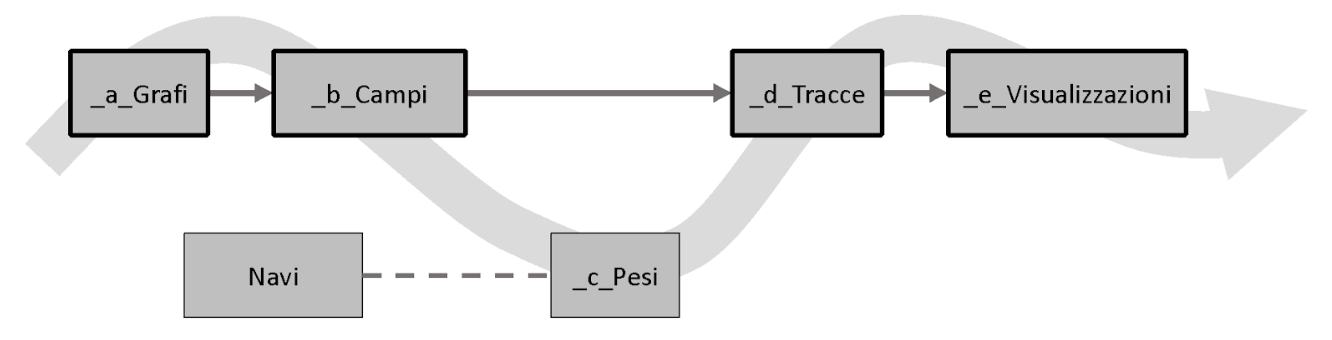
The blocks with the thicker frame must be run by the end-user. The other blocks should be edited for an advanced use of VISIR-2. The wavy arrow indicates the code flow.
The additional modules are automatically invoked by the primary ones. The advanced user can make use of the additional modules for further customizations.
In the VISIR-2 home folder, you will first notice the presence of three directories: __data, __namelist, __product
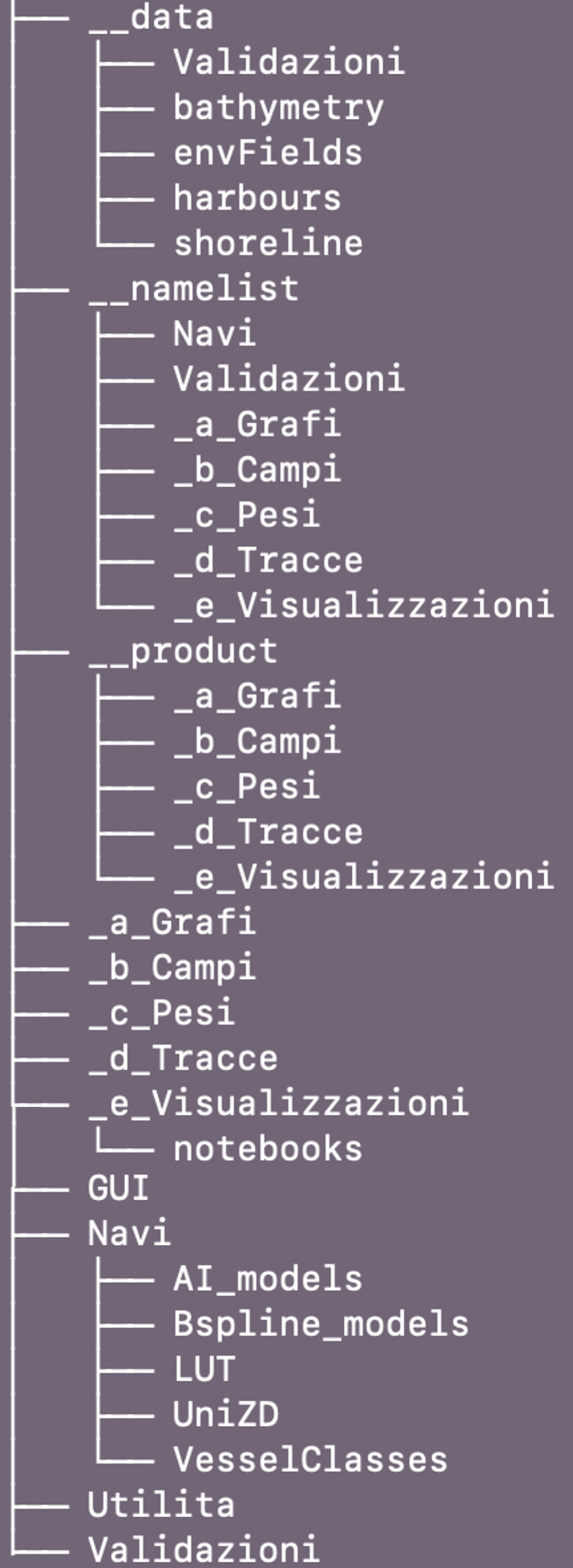
The first directory contains raw environmental data and a port code database, the second one includes namelists required to execute each VISIR-2 module, and the third one holds the outcomes of VISIR-2 processing. Additionally, the __product folder contains a copy of the actual namelists used for execution.
Both the __namelist and __product folders are organised into subfolders named after the main VISIR-2 modules: _a_Grafi, _b_Campi, _c_Pesi, _d_Tracce, _e_Visualizzazioni.
Each of the __namelist subfolders contains template_*.yaml files. The namelists of most modules include an option for performance profiling.
The core VISIR-2 outputs are located in __product/_d_Tracce/<run_folder>/ and are the following files:
Solutions.*: a table of key metrics for the selected routes*_voyageplan.*: set of files detailing the sequence of route waypoints, ship kinematics, and corresponding environmental information. A file exists for each optimization objective. The voyage plans are saved in both xml and json format.
Additionally, there are supplementary VISIR-2 modules: Navi, GUI, Utilita, Validazione. Each module includes a MAIN_*.py file where execution initiates and concludes. Main modules log their input conditions into specific yaml files, which are stored in the __product folder.
The VISIR-2 installation folder includes a Readme file and specifications for setting up and utilising the required virtual environment.
Additional details about the VISIR-2 modules are provided in the subsequent subsections. For more in-depth information, please refer to the reference paper on VISIR-2 in the Publications section.
_a_Grafi
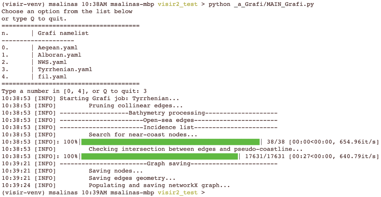
VISIR-2, like VISIR-1, is based on a graph-search method, making the availability of a graph a fundamental requirement for running the software. This module generates a graph using a given grid spatial resolution invDx and connectivity nu. The bathymetric map is utilised to account for under keel clearance of the vessel. Edges leading to navigation in overly shallow waters (i.e., with a depth lower than maxDraught) are pruned. A console output from _a_Grafi is shown below.
_b_Campi
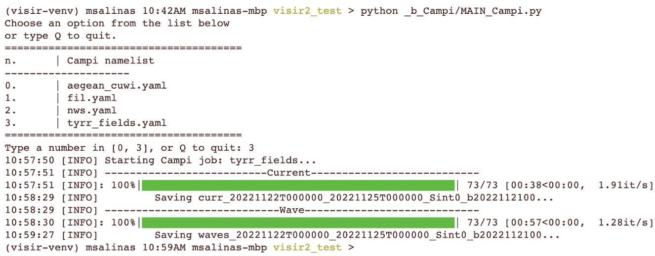
The purpose of this module is to perform spatial interpolation of environmental fields across the graph grid. Users can choose the fields of interest (such as waves, currents, or winds) and specify the desired spatial interpolation method (either calculating the mean of edge head/tail field values or using bilinear interpolation at the edge barycentre) through the Sint parameter. The beginning of the console output of _b_Campi is shown here.
_c_Pesi
This module is responsible for evaluating the edge weights to be subsequently used by the shortest path algorithm in _d_Tracce. These weights include sailing time and CO2 mass flow. Sailing time depends on both edge length and vessel speed. The latter is determined by the vessel performance model (provided by the Navi module) and the actual environmental conditions. It is important to note that manually running the _c_Pesi module is not required, as it is automatically invoked during the execution of _d_Tracce.
_d_Tracce
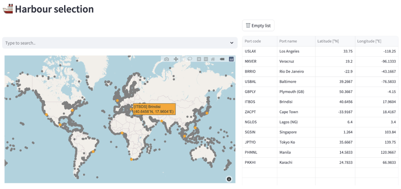
This module is responsible for calculating the shortest paths, producing routes with the least length, duration, or CO2 emissions. To utilise this module, users must specify the vessel under consideration, departure and arrival locations of the route, departure date and time, the environmental fields to be considered, the designated graph. The departure and arrival locations can be specified either by geographical coordinates or by international seaport codes. The latter can be found through the GUI launched by MAIN_search_harbours_DB.py as shown below.
The console output of _d_Tracce appears like this:
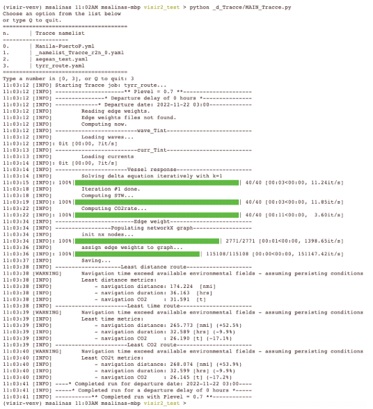
This module generates an output file, Solutions.csv, containing metrics for the optimal routes, and other files corresponding to voyage plans in various formats.
The two formats employed by VISIR-2 for storing voyage plans across different routes are selected based on their complementary features. The XML output facilitates rich metadata and adheres to strict schema validation, making it a potential candidate for evolving into a standard format for route exchange. On the other hand, the JSON output, being less verbose, is better suited for human readability. It serves as a standard format in various environments, including the pandas library in Python. A JSON-to-RTZ conversion library is also available in the VISIR-2 Zenodo community.
_e_Visualizzazioni
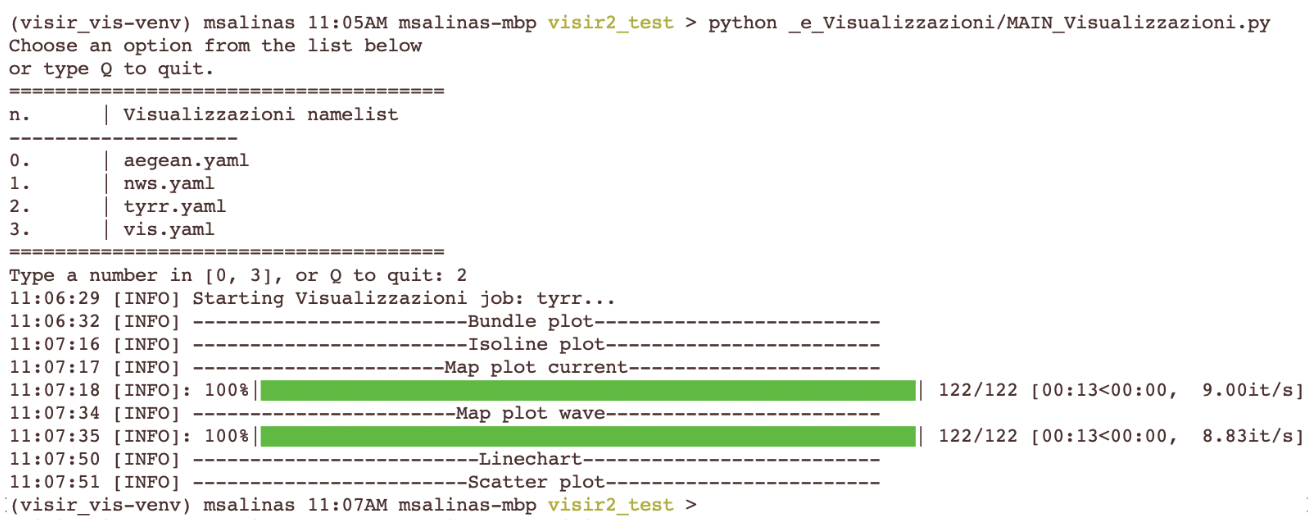
This VISIR-2 module is responsible for presenting its results in graphical formats. It encompasses several common visualisation types: a georeferenced map displaying optimal routes and environmental fields, linecharts illustrating the sequence of vessel or sea values along the routes, and scatter diagrams offering an overview of key metrics for multiple routes in a two-dimensional space with colour coding. Additionally, in _e_Visualizzazioni/notebooks/, we provide a Jupyter notebook for generating the figures and tables in the results section of reference paper. These visuals and tables necessitate input datasets provided at https://doi.org/10.5281/zenodo.8233874 The console output of _e_Visualizzazioni may appear as shown here:
Navi
The namelist within the Navi module serves as an interface for selecting the specific vessel performance model to be employed in the computations of _c_Pesi and subsequent modules. Users have the option to either choose a pre-computed vessel response function from a range of providers or identify a new response function from an user-provided LUT. The names of the pre-computed models (i.e., those used also in the paper listed in the references of this documentation) read either unige_* or unizd_*.
If a new model is to be identified:
-
Provide a LUT in the form of a csv file, with the following headers (case sensitive!):
- If sailboat:
Vw alpha STW leeway wind velocity in knots true relative wind angle, corresponds to δi speed through water in knots leeway velocity in knots 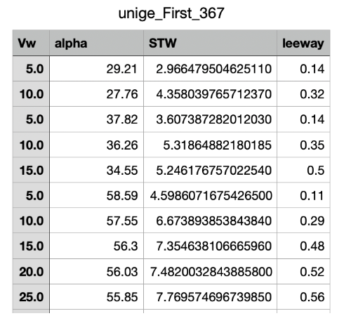
- If motorboat:
Hs alpha Load STW CO2rate significant wave height in metres true relative wave angle, corresponds to δa engine load factor in % speed through water in knots CO2 emission rates in tons per hour -
In Navi/MAIN_vesselModels_identify.py, specify the following variables:
vessel_type(either motor or sail)LUT_base_dirfilename
-
Run Navi/MAIN_vesselModels_identify.py. This generates:
__namelist/Navi/extra_<filename>.yamlNavi/Bspline_models/extra_<filename>/*.bsplineNavi/LUT/extra_<filename>.csv
Validation
The validation of the VISIR-2 integrity can be initiated using the Validazioni module. It is designed to conduct multiple tests and compare their results against established oracles. The testbed encompasses both analytical solutions of the shortest path problem in idealised environmental conditions and benchmark runs. After executing the testbed, the module provides an assertion regarding whether the test was passed or not. This assertion is crucial for identifying any critical alterations in the software’s functionality that may have resulted from code developments. This is why it is recommended to execute Validazioni before running a version of VISIR-2 which has undergone substantial modifications.